API Reference

class outflowpy.input.Input(br, nr, rss, corona_temp=None, mf_constant=None, sound_speed=None, polynomial_coeffs=None, polynomial_type='smooth_monotonic')

Bases: object

Input to PFSS/outflow field modelling.

Parameters:

br (sunpy.map.GenericMap) – Boundary condition of radial magnetic field at the inner surface. Note that the data must have a cylindrical equal area projection.
nr (int) – Number of cells in the radial direction on which to calculate the 3D solution.
rss (float) – Radius of the source surface, in units of solar radius
(optional) (polynomial_type) – Temperature of the corona for the implicit solar wind solution (in K, see paper for details)
(optional) – Magnetofrictional constant factor
(optional) – Sound speed of the parker solution in km/s
(optional) – coefficients of the specified polynomial outflow profile
(optional) – One of ‘abs’, ‘clip’, ‘raw’, ‘smooth’ or ‘smooth_monotonic’. See the example scripts for details.

Notes

The input must be on a regularly spaced grid in \(\phi\) and \(s = \cos (\theta)\). See outflowpy.grid for more information on the coordinate system.

There are various options for calculating the outflow speed profile. If no extra arguments are provided, then the optimum profile for matching eclipse photographs is used. Alternatively:

If mf_constant = 0.0, then a PFSS solution is calculated. If mf_constant != 0.0 and either of corona_temp or sound_speed is specified, a Parker wind profile is calculated based on these parameters. If polynomial_coeffs are specified, the profile is calculated as a polynomial with these coeficcients. Polynomial_type determines how this polynomial is transformed to ensure it is nonnegative. See examples for details.

property grid: ~outflowpy.grid.Grid that the PFSS solution for this input is calculated on.

property map: sunpy.map.GenericMap representation of the input.

class outflowpy.output.Output(br, bs, bp, grid, input_map=None)

Bases: object

Output of outflow/PFSS calculations.

Parameters:

br – Magnetic field strengths in radial direction.
bs – Magnetic field strengths in elevation direction.
bp – Magnetic field strengths in azimuth direction.
grid (Grid) – Grid that the output was caclulated on.
input_map (sunpy.map.GenericMap) – The input map.

Notes

Instances of this class are intended to be created by outflowpy.outflow or `outflowpy.pfss’, and not by users.

get_bvec(coords, out_type='spherical')

Interpolate magnetic vectors at arbitrary coordinates.

Parameters:

coords (astropy.coordinates.SkyCoord) – An arbitary point or set of points (length N >= 1) in the PFSS model domain (1Rs < r < Rss).
out_type (str) – Takes values ‘spherical’ (default) or ‘cartesian’ and specifies whether the output vector is in spherical coordinates (B_r, B_theta, B_phi) or cartesian (B_x, B_y, B_z).

Returns:

bvec – (N, 3) shaped Quantity of magnetic field vectors.

Return type:

astropy.units.Quantity

Notes

The output coordinate system is defined by the input magnetogram with x-z plane equivalent to the plane containing the Carrington meridian (0 deg longitude)

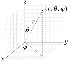
The spherical coordinates follow the physics convention: https://upload.wikimedia.org/wikipedia/commons/thumb/4/4f/3D_Spherical.svg/240px-3D_Spherical.svg.png) Therefore the polar angle (theta) is the co-latitude, rather than the latitude, with range 0 (north pole) to 180 degrees (south pole)

The conversion which relates the spherical and cartesian coordinates is as follows:

\[B_R = sin\theta cos\phi B_x + sin\theta sin\phi B_y + cos\theta B_z\]

\[B_\theta = cos\theta cos\phi B_x + cos\theta sin\phi B_y - sin\theta B_z\]

\[B_\phi = -sin\phi B_x + cos\phi B_y\]

The above equations may be written as a (3x3) matrix and inverted to retrieve the inverse transformation (cartesian from spherical)

trace(tracer, seeds)

Trace magnetic field lines.

Parameters:

tracer (tracing.Tracer) – Field line tracer.
seeds (astropy.coordinates.SkyCoord) – Starting coordinates.

property bc

B on the centres of the cell faces.

Returns:

br (astropy.units.Quantity) – A nphi, ns, nrho + 1 shaped Quantity.
btheta (astropy.units.Quantity) – A nphi, ns + 1, nrho shaped Quantity.
bphi (astropy.units.Quantity) – A nphi + 1, ns, nrho shaped Quantity.

Notes

The three components are not co-located at the same locations. Component n is located on cell faces of constant n, e.g. the r component is located on the cell faces at constant r values.

property bcx

B on the centres of the cell faces PLUS ghost points.

Returns:

br (astropy.units.Quantity) – A nphi+2, ns+2, nrho + 1 shaped Quantity.
btheta (astropy.units.Quantity) – A nphi+2, ns + 1, nrho+2 shaped Quantity.
bphi (astropy.units.Quantity) – A nphi + 1, ns+2, nrho+2 shaped Quantity.

Notes

The three components are not co-located at the same locations. Component n is located on cell faces of constant n, e.g. the r component is located on the cell faces at constant r values.

property bg

B as a (weighted) averaged on grid points.

Returns:: A (nphi + 1, ns + 1, nrho + 1, 3) shaped Quantity. The last index gives the corodinate axis, 0 for Bphi, 1 for Bs, 2 for Brho. Because the phi dimension is periodic, bg[0, :, :] == bg[-1, :, :].
Return type:: astropy.units.Quantity

property bunit

~astropy.units.Unit of the input map data.

If no metadata is available, returns dimensionless units.

property coordinate_frame

Coordinate frame of the input map.

Notes

This is either a ~sunpy.coordinates.frames.HeliographicCarrington or ~sunpy.coordinates.frames.HeliographicStonyhurst frame, depending on the input map.

property coords_x

Extended coordinates at cell faces.

Return type:: rcx, scx, pcx

property dtime: Date and time of the input map.

property source_surface_br

Radial magnetic field component on the source surface.

Return type:: sunpy.map.GenericMap

property source_surface_pils

Coordinates of the polarity inversion lines on the source surface.

Notes

This is always returned as a list of ~astropy.coordinates.SkyCoord, as in general there may be more than one polarity inversion line.

Code for calculating a PFSS extrapolation.

outflowpy.pfss.pfss(input)

Compute PFSS field using the code from pfsspy.

Extrapolates a 3D PFSS using an eigenfunction method in \(r,s,p\) coordinates, on the dumfric grid (equally spaced in \(\rho = \ln(r/r_{sun})\), \(s= \cos(\theta)\), and \(p=\phi\)).

Parameters:: input (Input) – Input parameters.
Returns:: out
Return type:: Output

Notes

In order to avoid numerical issues, the monopole term (which should be zero for a physical magnetic field anyway) is explicitly excluded from the solution.

The output should have zero current to machine precision, when computed with the DuMFriC staggered discretization.

Pure python code for calculating outflow fields. Using coordinates and naming conventions from pfsspy, for compatibility with that module

outflowpy.outflow.outflow(input, existing_fname=None)

Compute outflow field using the precompiled Fortran routine – much faster than the python alternative.

Extrapolates a 3D outflow field using an eigenfunction method in \(r,s,p\) coordinates, on the dumfric grid (equally spaced in \(\rho = \ln(r/r_{sun})\), \(s= \cos(\theta)\), and \(p=\phi\)).

Parameters:: input (Input) – Input parameters.
Returns:: out
Return type:: Output

outflowpy.outflow.outflow_python(input)

Compute outflow field using pure Python routines.

Extrapolates a 3D outflow field using an eigenfunction method in \(r,s,p\) coordinates, on the dumfric grid (equally spaced in \(\rho = \ln(r/r_{sun})\), \(s= \cos(\theta)\), and \(p=\phi\)).

Parameters:

input (Input) – Input parameters.

Returns:

out (Output)
The output should have zero current to machine precision,
when computed with the DuMFriC staggered discretization.

class outflowpy.tracing.FastTracer(max_steps='auto', step_size=1)

Bases: Tracer

FastTracer uses Fortran routines in the native spherical coordinate system (rather than tracing in cartesian coordinates and transforming as for the other tracers), so works well at/near the poles. Also includes the option to save out a synthetic ‘image’ matrrix rather than the field lines themselves.

Parameters:

max_steps (str, int) –
Maximum number of steps each streamline can take before stopping. This controls the total amount of memory allocated for all the streamlines.

If 'auto' (the default) this is set to \(4n_{r} / ds\), where \(n_{r}\) is the number of radial grid points and \(ds\) is the specified step_size.
step_size (float) – Step size as a fraction of numerical grid cell size at the equator. Must be less than the number of radial coordinate cells.

trace(seeds, output, generate_image=False, save_flag=True, parameters=None, image_resolution=500, image_extent=None)

Parameters:

seeds (astropy.coordinates.SkyCoord) – Coordinaes of the magnetic field seed points.
output (outflowpy.Output) – Outflow field output.
(optional) (save_flag) – Array of shape (4,) specifying the parameters (see Paper II) for image generation. If None will use default values
(optional) – The resolution of the generated image matrix in both dimentions
(optional) – The altitude of the extent of the image matrix. If None, will be set to the source surface height
(optional) – If True, outputs an image matrix
(optional) – If True, outputs the field line coordinates. Unwise for many field lines as this takes a lot of memory.

Returns:

streamlines (FieldLines) – Traced field lines. If save_flag = False will only output one field line.
image_matrix (numpy.ndarray) – Matrix of the generated image values, shape (image_resolution, image_resolution). Only produced if generate_image=True.

class outflowpy.tracing.FortranTracer(max_steps='auto', step_size=1)

Bases: Tracer

Tracer using Fortran code.

Parameters:

max_steps (str, int) –
Maximum number of steps each streamline can take before stopping. This controls the total amount of memory allocated for all the streamlines.

If 'auto' (the default) this is set to \(4n_{r} / ds\), where \(n_{r}\) is the number of radial grid points and \(ds\) is the specified step_size.
step_size (float) – Step size as a fraction of numerical grid cell size at the equator. Must be less than the number of radial coordinate cells.

Notes

Because the stream tracing is done in spherical coordinates, there is a singularity at the poles (ie. \(s = \pm 1\)), which means seeds placed directly on the poles will not go anywhere.

trace(seeds, output)

Parameters:

seeds (astropy.coordinates.SkyCoord) – Coordinaes of the magnetic field seed points.
output (outflowpy.Output) – outflow field output.

Returns:

streamlines – Traced field lines.

Return type:

FieldLines

static vector_grid(output): Create a streamtracer.VectorGrid object from an ~outflowpy.Output.

class outflowpy.tracing.PythonTracer(atol=0.0001, rtol=0.0001)

Bases: Tracer

Tracer using native python code.

Uses scipy.integrate.solve_ivp, with an LSODA method.

trace(seeds, output)

Parameters:

seeds (astropy.coordinates.SkyCoord) – Coordinaes of the magnetic field seed points.
output (outflowpy.Output) – outflow field output.

Returns:

streamlines – Traced field lines.

Return type:

FieldLines

class outflowpy.tracing.Tracer

Bases: ABC

Abstract base class for a streamline tracer.

static cartesian_to_coordinate(): Convert cartesian coordinate outputted by a tracer to a FieldLine object.

static coords_to_xyz(seeds, output)

Given a set of astropy sky coordinates, transoform them to cartesian x, y, z coordinates.

Parameters:

seeds (astropy.coordinates.SkyCoord) –
output (outflowpy.Output) –

static validate_seeds(seeds): Check that seeds has the right shape and is the correct type.

outflowpy.utils.carr_cea_wcs_header(dtime, shape, *, map_center_longitude=<Quantity 0. deg>)

Create a Carrington WCS header for a Cylindrical Equal Area (CEA) projection. See [1] for information on how this is constructed.

Parameters:

dtime (datetime, None) – Datetime to associate with the map.
shape (tuple) – Map shape. The first entry should be number of points in longitude, the second in latitude.
map_center_longitude (astropy.units.Quantity) – Change the world coordinate longitude of the central image pixel to allow for different roll angles of the Carrington map. Default to 0 deg. Must be supplied with units of astropy.units.deg

References

outflowpy.utils.equal_seed_sampler(output, nseeds, r_start)

Returns equally distributed seeds in the plane of view, at a given altitude r_start.

Returns:: seeds – List of coordinates in the astropy coordinate format.
Return type:: SkyCoord object

outflowpy.utils.find_eclipse_time(eclipse_year)

Find the eclipse date corresponding to the specified year (of the 12 eclipses considered in our paper, 2006-2024). Returns an error if an unsuitable year is requested. This function will likely be improved in future releases.

Parameters:: eclipse_year (int) – Year of the desired eclipse
Returns:: date – Date of eclipse. Format is YYYY-MM-DDT00:00:00
Return type:: string

outflowpy.utils.is_cea_map(m, error=False)

Returns True if m is in a cylindrical equal area projeciton.

Parameters:

m (sunpy.map.GenericMap) –
error (bool) – If True, raise an error if m is not a CEA projection.

outflowpy.utils.is_full_sun_synoptic_map(m, error=False)

Returns True if m is a synoptic map spanning the solar surface.

Parameters:

m (sunpy.map.GenericMap) –
error (bool) – If True, raise an error if m does not span the whole solar surface.

outflowpy.utils.load_sampled_seeds(output, nseeds, fname=None, thomson_weighting=True)

Loads an existing randomly-generated selection of seeds, to be used for generating consistent plots etc. Outputs are weighted based on the Thomson scattering factor (this may later become optional)

Parameters:

output (output object) – Output object from the outflow field or pfss calculation
nseeds (int) – Number of field line seeds (takes the first nseeds from the sample)
(optional) (thomson_weighting) – File name for sample seed location
(optional) – If True, weights the field line locations based on their Thomson Scattering angle. If False, starts the field line locations at right angles to the view angle.

Returns:

seeds – List of coordinates in the astropy coordinate format.

Return type:

SkyCoord object

outflowpy.utils.plane_seed_sampler(output, nseeds, r_skew, rss)

Returns a list of sampled seeds for use in the field line tracer, ‘randomly’ distributed according to the latin hypercube method and weighted radially. Returns seeds weighted by their significance based on the Thomson Scattering effect, rather than randomly in the direction of view.

Parameters:

output (output object) – Output object from the outflow field or pfss calculation
nseeds (int) – Number of field line seeds
r_skew (float) – Skew factor towards more seeds being selected lower in the domain. Set to zero for no skew.
rss (float) – Maximum altitude of sampled seeds (can be lower than the source-surface height)

Returns:

seeds – List of coordinates in the astropy coordinate format.

Return type:

SkyCoord object

outflowpy.utils.random_seed_sampler(output, nseeds, r_skew, rss)

Returns a list of sampled seeds for use in the field line tracer, ‘randomly’ distributed according to the latin hypercube method and weighted radially.

Parameters:

output (output object) – Output object from the outflow field or pfss calculation
nseeds (int) – Number of field line seeds
r_skew (float) – Skew factor towards more seeds being selected lower in the domain. Set to zero for no skew.
rss (float) – Maximum altitude of sampled seeds (can be lower than the source-surface height)

Returns:

seeds – List of coordinates in the astropy coordinate format.

Return type:

SkyCoord object

outflowpy.obtain_data.download_hmi_mdi_crot(crot_number, source=None, use_cached=False, cache_dir=None, scale_hmi=True)

Downloads the raw HMI data with Carrington rotation number ‘crot_number’.

Parameters:

crot_number (int) – Carrington rotation number.
(optional) (scale_hmi) – If specified, ensures that the data comes from either ‘MDI’ or ‘HMI’. This stops a mismatch if the maps are stitched together.
(optional) – If True, will attempt to find cached data, and if it doesn’t exist will instead download and save it
(optional) – Directory in which to save cached downloads. If None, will save to ./_download_cache.
(optional) – If True, scales the HMI data such that they are calibrated to MDI.

Returns:

data (array)
Array corresponding to the magnetic field strength on the solar surface
header (sunpy.header object)
Object containing some metadata about the downloaded data. May not be quite accurate.

Notes

If the specified rotation is less than 2098, the data downloaded willl be from MDI. If not, HMI. This information will hopefully be contained within the header so it can be ‘corrected’ in due course. The output here will not be smoothed in time, leading to a discontinuity on the far side of the sun. If this is undesirable, specify an observation time instead.

outflowpy.obtain_data.prepare_hmi_mdi_crot(crot_number, ns_target, nphi_target, smooth=0.0, use_cached=False, cache_directory=None)

Downloads (without email etc.) the HMI or MDI data matching the specified rotation number, applies smoothing using legendre polynomials and interpolates to a new grid size

Parameters:

crot_number (int) – Carrington rotation number.
ns_target (int) – Target number of grid cells in latitudinal direction.
nphi_target (int) – Target number of grid cells in longitudinal direction.
smooth (float) – Smoothing factor for the data interpolation.
(optional) (cache_dir) – If True, will attempt to find cached data, and if it doesn’t exist will instead download and save it.
(optional) – Directory in which to save cached downloads. If None, will save to ./_download_cache.

Returns:

data (sunpy.map.Map)
A sunpy map object corresponding to the requested rotation number

Notes

Must be in the allowable range of Carrington rotations. Outputs a sunpy map object

outflowpy.obtain_data.prepare_hmi_mdi_time(obs_time, ns_target, nphi_target, smooth=0.0, use_cached=False, cache_directory=None, interpolate_synoptic_maps=True)

Downloads (without email etc.) the HMI or MDI data corresponding to the specified time Obtains three HMI/MDI magnetograms and stiches them together as appropriate. Then applies smoothing etc. as for the single crot script.

Parameters:

obs_time (string) – String corresponding to the observation time. Format is YYYY-MM-DDThh:mm:ss
ns_target (int) – Target number of grid cells in latitudinal direction.
nphi_target (int) – Target number of grid cells in longitudinal direction.
smooth (float) – Smoothing factor for the data interpolation.
(optional) (interpolate_synoptic_maps) – If True, will attempt to find cached data, and if it doesn’t exist will instead download and save it.
(optional) – Directory in which to save cached downloads. If None, will save to ./_download_cache.
(optional) – If True, will use the synoptic maps either side of the observation time to smooth the data in time, removing discontinutities and allowing for flux emergence.

Returns:

data (sunpy.map.Map)
A sunpy map object corresponding to the requested time

Notes

Must be in the allowable range of Carrington rotations Outputs a sunpy map object

outflowpy.obtain_data.sh_smooth(raw_data, smooth, ns_target, nphi_target, cutoff=10)

Parameters:

f (array) – Input array representing the radial magnetic field on the solar surface. Designed to be an import from HMI or equivalent
smooth (real) – Smoothing coefficient. Set to zero to include everything, and increase to increase the amount of blurring
cutoff (integer) – The largest value of smooth*l(l+1) that will be considered. Everything else will be set to zero.

Returns:

f – The smoothed version of the input array.

Return type:

array

Notes

This implementation uses discrete eigenfunctions (in latitude) instead of Plm.

Parameters: smooth – coefficient of filter exp(-smooth * lam) [set cutoff=0 to include all eigenvalues. This is quicker for small matrices.] cutoff – largest value of smooth*lam to include [so 10 means ignore blm multiplied by exp(-10)]