Download and plot HMI/MDI data

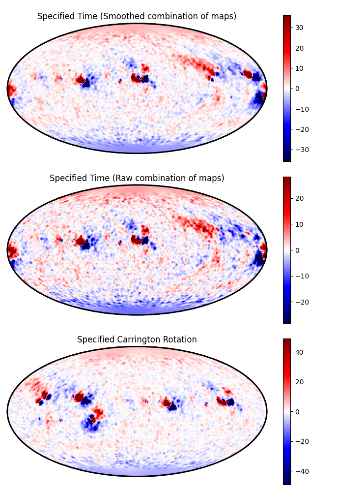
This example downloads the data for either a specified time (of the 2017 eclipse) or for a specified Carrington Rotation, and plots the input data on a Mollweide projection.

import outflowpy

import matplotlib.pyplot as plt
import numpy as np


#Specify resolutions for the input (nrho doesn't matter in this case, as only care about the lower boundary data)
ns = 180
nphi = 360
nrho = 60

#Specify observation time
obs_time = "2017-08-21T00:00:00"

#Download and prepare the data for this time
hmi_map_time = outflowpy.obtain_data.prepare_hmi_mdi_time(obs_time, ns, nphi, smooth = 1.0*5e-2/nphi, use_cached = True)
hmi_map_time_raw = outflowpy.obtain_data.prepare_hmi_mdi_time(obs_time, ns, nphi, smooth = 1.0*5e-2/nphi, use_cached = True, interpolate_synoptic_maps=False)
hmi_map_crot = outflowpy.obtain_data.prepare_hmi_mdi_crot(2194, ns, nphi, smooth = 1.0*5e-2/nphi, use_cached = True)

#Create the Input objects. Outflow profile doesn't matter so just specify PFSS.
outflow_in_time = outflowpy.Input(hmi_map_time, nrho, 2.5, mf_constant = 0.0)
outflow_in_time_raw = outflowpy.Input(hmi_map_time_raw, nrho, 2.5, mf_constant = 0.0)
outflow_in_crot = outflowpy.Input(hmi_map_crot, nrho, 2.5, mf_constant = 0.0)

#Define the plotting function
def plot_boundary_data(ax, data, title):
    lon_edges = np.linspace(-np.pi, np.pi, nphi+1)
    lat_edges = np.arccos(np.linspace(1., -1., ns+1)) - np.pi/2
    vmax = np.percentile(data, 99.5)
    im = ax.pcolormesh(lon_edges, lat_edges, data, vmin = -vmax, vmax = vmax, cmap = 'seismic', rasterized=True)
    ax.patch.set_linewidth(2)
    ax.patch.set_edgecolor("black")

    for spine in ax.spines.values():
        spine.set_edgecolor("black")
        spine.set_linewidth(2)

    ax.set_xticks([])
    ax.set_yticks([])
    plt.colorbar(im)

    ax.set_title(title)

    return

#Plot this boundary data
fig, axs = plt.subplots(3,1, subplot_kw = {"projection": "mollweide"}, figsize = (6.9, 10.0))

ax = axs[0]
plot_boundary_data(ax, outflow_in_time.br, 'Specified Time (Smoothed combination of maps)')
ax = axs[1]
plot_boundary_data(ax, outflow_in_time_raw.br, 'Specified Time (Raw combination of maps)')
ax = axs[2]
plot_boundary_data(ax, outflow_in_crot.br, 'Specified Carrington Rotation')



plt.tight_layout()
plt.show()

Expected output: