Outflow Speed Comparison

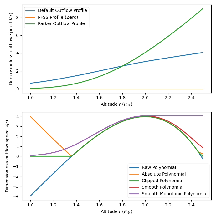
This example shows the various methods for generating outflow profiles and plots them

import outflowpy

import matplotlib.pyplot as plt
import numpy as np
from astropy.time import Time
import sunpy.map

#Model resolution
ns = 90
nphi = 180
nrho = 60
#Source-surface height (in solar radii)
rss = 2.5

#Analytic lower boundary condition. This is necessary as the Input class requires a map, and using a dipole is faster than downloading data
phi = np.linspace(0, 2 * np.pi, nphi)
s = np.linspace(-1, 1, ns)
s, phi = np.meshgrid(s, phi)
def dipole_Br(r, s):
    return s**7
br = dipole_Br(1, s)

#Create sunpy headers for this analytic data (when downloading real data this is more meaningful)
header = outflowpy.utils.carr_cea_wcs_header(Time('2020-1-1'), br.shape)
input_map = sunpy.map.Map((br.T, header))

#Generate outflow profiles using defaults or Parker
fig, axs = plt.subplots(2,1, figsize = (6.9, 7.0))

ax = axs[0]
#Default profile (optimised for field line shapes)
outflow_in_default = outflowpy.Input(input_map, nrho, rss)
#PFSS solution (zero outflow)
outflow_in_pfss = outflowpy.Input(input_map, nrho, rss, mf_constant = 0.0)
#Parker solution with specified sound speed in m/s
outflow_in_parker = outflowpy.Input(input_map, nrho, rss, mf_constant = 5e-17, sound_speed = 125e3)

ax.plot(np.exp(outflow_in_default.grid.rg), outflow_in_default.vg, label = "Default Outflow Profile", linewidth = 2.)
ax.plot(np.exp(outflow_in_pfss.grid.rg), outflow_in_pfss.vg, label = "PFSS Profile (Zero)", linewidth = 2.)
ax.plot(np.exp(outflow_in_parker.grid.rg), outflow_in_parker.vg, label = "Parker Outflow Profile", linewidth = 2.)

ax.set_xlabel('Altitude $r$ ($R_\odot$)')
ax.set_ylabel('Dimensionless outflow speed $V_(r)$')
ax.legend()

#Generate outflow profiles using specified polynomials
ax = axs[1]
#Specify polynomial coefficients (these are unrealistically picked merely to illustrate the differences between the types)
coeffs = [-14, 8, 1.5, 1.5, -1.0]
#Raw polynomial (will create errors if negative -- as this does)
outflow_in_raw = outflowpy.Input(input_map, nrho, rss, polynomial_coeffs = coeffs, polynomial_type = 'raw')
#Absolute value of the polynomial
outflow_in_abs = outflowpy.Input(input_map, nrho, rss, polynomial_coeffs = coeffs, polynomial_type = 'abs')
#Clipped polynomial
outflow_in_clip = outflowpy.Input(input_map, nrho, rss, polynomial_coeffs = coeffs, polynomial_type = 'clip')
#Smooth polynomial
outflow_in_smooth = outflowpy.Input(input_map, nrho, rss, polynomial_coeffs = coeffs, polynomial_type = 'smooth')
#Smooth monotonic polynomial
outflow_in_smooth_monotone = outflowpy.Input(input_map, nrho, rss, polynomial_coeffs = coeffs, polynomial_type = 'smooth_monotonic')

ax.plot(np.exp(outflow_in_raw.grid.rg), outflow_in_raw.vg, label = "Raw Polynomial", linewidth = 2.)
ax.plot(np.exp(outflow_in_abs.grid.rg), outflow_in_abs.vg, label = "Absolute Polynomial", linewidth = 2.)
ax.plot(np.exp(outflow_in_clip.grid.rg), outflow_in_clip.vg, label = "Clipped Polynomial", linewidth = 2.)
ax.plot(np.exp(outflow_in_smooth.grid.rg), outflow_in_smooth.vg, label = "Smooth Polynomial", linewidth = 2.)
ax.plot(np.exp(outflow_in_smooth_monotone.grid.rg), outflow_in_smooth_monotone.vg, label = "Smooth Monotonic Polynomial", linewidth = 2.)

ax.set_xlabel('Altitude $r$ ($R_\odot$)')
ax.set_ylabel('Dimensionless outflow speed $V_(r)$')
ax.legend()


plt.tight_layout()
plt.show()

Expected output: